|
Documentation
The Matlab functions and scripts in the MA toolbox are:
Some general comments:
All functions include a test case. If the function is called without arguments, this test will be run. It makes sense to play around with the parameters in the test case to understand them.
Most functions have an input argument called "p". This is a Matlab structure variable and is used to store all parameter values conveniently. See the test case on how to set them, in some cases default values are defined.
These functions require that the WAV (PCM) files are loaded into Matlab using "wavread ". If the original files are MP3s or similar formats, it is possible to decode them using Lame, Winamp (output plugin discwriter), Wavelab, etc.
This function applies some auditory models to estimate how strong the loudness sensation is per frequency band. The main parts are (1) outer-ear model, (2) critical-band rate scale (Bark-scale), (3) spectral masking, and (4) Sone. The computations (including references to the literature) are described e.g. in [3,4].
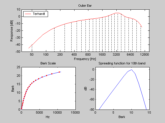
Figure 1. The main characteristics of the sone model. The upper subplot shows the width of the critical-bands and the outer-ear model. The lower left shows the relationship between the Bark-scale and Hz. The lower right shows the spectral masking function. Some things to notice: The Bark-scale is linear up to about 500Hz. The spectral masking is not symetric. Higher tones are masked stronger by lower ones than vice versa. The outer-ear is most responsive to frequencies around 3-4kHz. For details on the models see the source code (e.g. "type ma_sone").
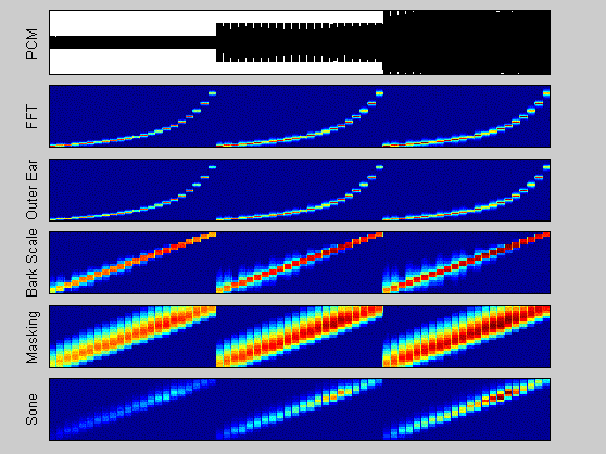
Figure 2. The characteristics of the sone model can be demonstrated with a simple sine-tone. The tone is generated at different frequencies (center frequencies of the critical-bands) with fixed amplitude (3 times, each time the fixed amplitude is increased). Note the difference between the linear frequency scale (used in the outer-ear and FFT representations) and the Bark-scale (the lower 3 subplots). The sinusoids in each sweep from low to high have the same amplitudes, they are not perceived equally loud (uncomment the "sound(wav,p.fs)" line in the test case code to hear the sound, this pitch dependent loudness sensation is reflected in the model (in contrast to the MFCC model).
Mel Frequency Cepstrum Coefficients are very popular in speech processing. They are based on the Mel-scale. The Mel scale is defined such that a tone of 1000Hz equals 1000mel. Different models for the Mel-scale exist, it is defined so that if tone A is perceived twice as high as tone B then its mel value is twice as high. (The Bark-scale and in particular the width of the critical-bands are defined by masking tresholds, i.e., how close can two tones be too each other on the frequency scale so that they are both perceived and one doesn't mask the other).
In addition to using the Mel-scale, dB values are computed and the spectrum is compressed (and smoothed) using a Discrete Cosine Transform (DCT). This compressed representation is well suited for computational heavy algorithms. (Note that a DCT compression could also be applied to the sonogram.)
Some questionable aspects are: (1) no outer-ear model is used, (2) the dB-SPL values are well known not to be a good representation for the loudness sensation, and (3) the smoothing (spectral masking) is not explicitly defined.

Figure 3. The basic model of the MFCCs. The upper subplot shows the filterbank of triangular filters. The lower subplot shows the Discrete Cosine Transform matrix.
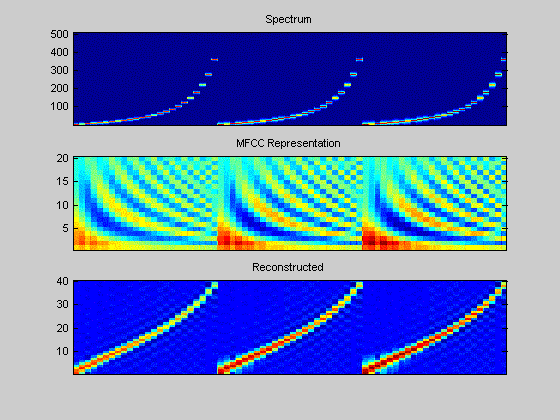
Figure 4. Using the same input sound as in Figure 2 the characteristics of the MFCC can be studied. Some things to notice: The mel-scale differs from the bark-scale (not line is not straight). The MFCCs don't consider characteristics of the outer-ear. Artefacts from the DCT transform are clearly visible.
The Spectrum Histogram is a very simple approach to summarize the variations in the dynamics. It counts for each frequency band how many times certain loudness levels are exceeded. The SH is described in [4].
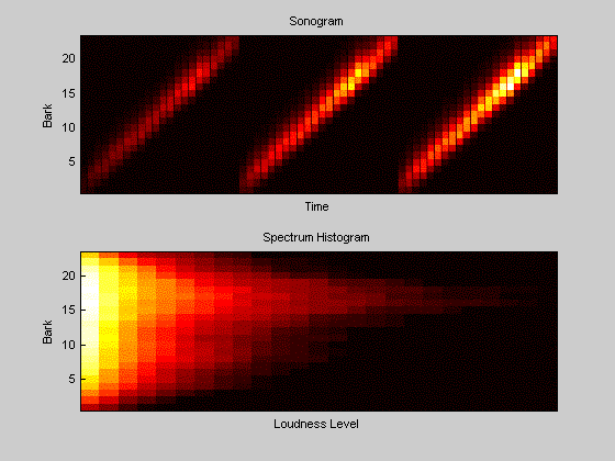
Figure 5. Same test sound as in the examples above. The spectrum histogram counts how often a loudness level was exceeded in each critical-band.
The Periodicity Histogram is based on a comb-filter and describes periodically reoccurring sharp attacks in the audio. Details are described in [4].
Although the PH is not a useful similarity measure it serves as a good starting point to compute various descriptors.
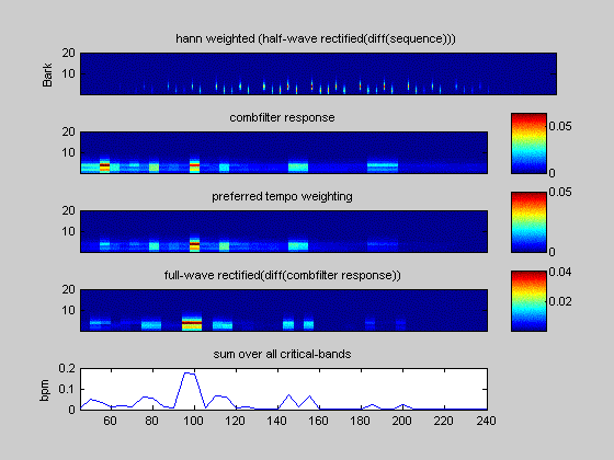
Figure 6. The different steps in computing the periodicities for a 12sec time frame. The input is a very simple test sound generated with "ma_test_create_wav".

Figure 7. If the input is long enough, then the results from each 12sec frame are summarized in a histogram, counting for each periodicity (bpm) how often specific energy levels were exceeded.
The Fluctuation Pattern is based on a model of the perceived fluctuation for amplitude modulated tones. Details can be found in [3].
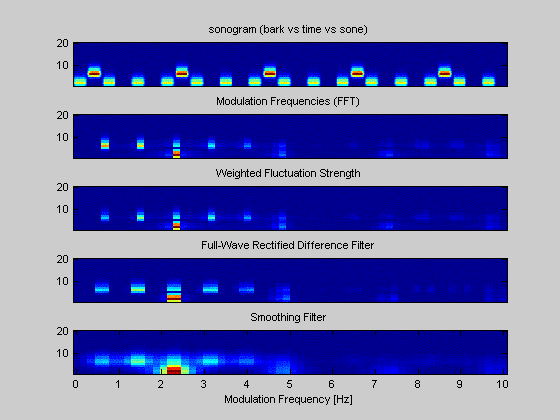
Figure 8. The different steps in computing the fluctuation pattern for a 6sec sequence.
Frame Clustering takes a frame based representation as input (e.g. MFCCs) and creates a cluster model. The cluster models can be compared to each other with "ma_cms" (Cluster Model Similarity).
A variation using the Earth Mover's Distance was originally published by Beth Logan and Ariel Salomon [1]. A second variation using monte carlo sampling was publised by Jean-Julien Aucouturier and Francois Pachet [2]. For a good overview of different parameters and optimum values see [5].
WARNING: although I tried to stick to the papers there are no guarantees that this implementation is identical to the implementations used in [1,2,5]!
To run "ma_fc" with the "gmm" (Gaussian Mixture Model) option, the directory of the Netlab toolbox must be added to the Matlab path (e.g. "addpath ../netlab").
For figures see "ma_cms".
Cluster Model Similarity takes the models computed by "ma_fc" as input and outputs a distance. There are basically two ways to compute the similarity: using the EMD-KL (Earth Movers Distance and Kullback Leibler Divergence) [1], or by Monte Carlo sampling [2].
WARNING: there is no guarantee that this implementation is identical to those used in [1,2]!
EMD-KL requires functions implemented by Yossi Rubner. Monte Carlo sampling requires the NETLAB toolbox.
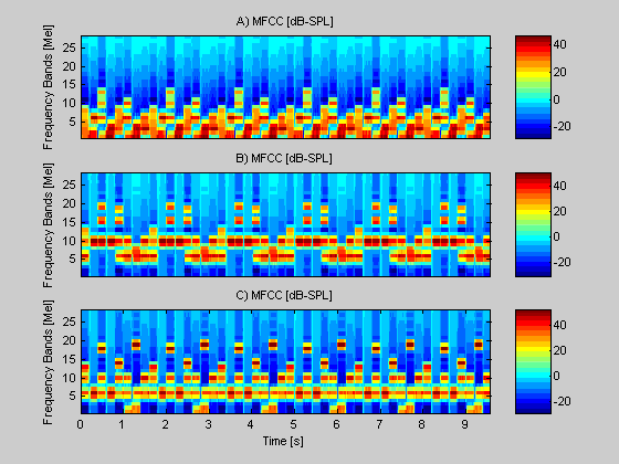
Figure 9. The three sounds used for this test case.

Figure 10. The cluster models can be visualized using "ma_cm_visu". In this case each sound was represented by 3 Gaussian clusters. The shapes and variances of each clusters (cummulated probability) are shown.
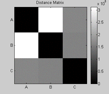
Figure 11. The distance matrix of the 3 sounds.

See "ma_cms" for figures.
This is a simple script to demonstrate how to combine the different functions if the goal is to evaluate different parameter settings. Input is a bunch of wav files sorted into directories such that similar pieces are in the same directory. At the end the R-precision is computed.
This is a simple script to demonstrate how the SOM toolbox (GNU-GPL) and the SDH toolbox (GNU-GPL) can be used to create "islands of music". (Both toolboxes need to be in the Matlab path.)
Questions, comments, feedback? Please contact: elias@oefai.at.
| - ma_sone | wav (PCM) to sone (specific loudness sensation) | |
| - ma_mfcc | wav (PCM) to MFCCs (Mel Frequency Cepstrum Coefficients) | |
| - ma_sh | sone to Spectrum Histogram | |
| - ma_ph | sone to Periodicity Histogram | |
| - ma_fp | sone to Fluctuation Pattern | |
| - ma_fc | frame based representation (MFCCs or sone) to cluster model (Frame Clustering) | |
| - ma_cms | cluster models to distance (Cluster Model Similarity) | |
| - ma_kmeans | kmeans clustering (used by "ma_fc") | |
| - ma_cm_visu | visualize a cluster model (as returned by "ma_fc") | |
| - ma_simple_eval | script for a simple evaluation of similarity measures | |
| - ma_simple_iom | script for a simple islands of music interface | |
Some general comments:
All functions include a test case. If the function is called without arguments, this test will be run. It makes sense to play around with the parameters in the test case to understand them.
Most functions have an input argument called "p". This is a Matlab structure variable and is used to store all parameter values conveniently. See the test case on how to set them, in some cases default values are defined.
These functions require that the WAV (PCM) files are loaded into Matlab using "wavread ". If the original files are MP3s or similar formats, it is possible to decode them using Lame, Winamp (output plugin discwriter), Wavelab, etc.
-- ma_sone -- |
This function applies some auditory models to estimate how strong the loudness sensation is per frequency band. The main parts are (1) outer-ear model, (2) critical-band rate scale (Bark-scale), (3) spectral masking, and (4) Sone. The computations (including references to the literature) are described e.g. in [3,4].
Compute sonogram for a pcm signal.

   [sone, Ntot, p] = ma_sone(wav,p)


USAGE

  ma_sone;                %% uses test-sound and creates figures

  sone = ma_sone(wav,p);  %% normal usage

  [sone, Ntot, p] = ma_sone(wav,p);


INPUT

  wav (vector) obtained from wavread (use mono input! 11kHz recommended)

  p (struct) parameters e.g.

   p.fs          = 11025;     %% sampling frequency of given wav (unit: Hz)

 * p.do_visu     = 0;         %% create some figures

 * p.do_sone     = 1;         %% compute sone (otherwise dB)

 * p.do_spread   = 1;         %% apply spectral masking

 * p.outerear = 'terhardt';   %% outer ear model {'terhardt' | 'none'}

 * p.fft_size = 256;          %% window size (unit: samples) 256 are ~23ms @ 11kHz

 * p.hopsize  = 128;          %% fft window hopsize (unit: samples)

 * p.bark_type   = 'table';   %% type of bark scale to use (either:

                              %% 'table' lookup (=default) with max 24 bands

                              %% (for 44kHz), or vector [min_freq max_freq num_bands]

 * p.dB_max      = 96;        %% max dB of input wav (for 16 bit input 96dB is SPL)

 all fields marked with * are optional (defaults are defined)


OUTPUT

  sone (matrix) rows are bark bands, columns are time intervalls,

                values are sone (or dB)

  Ntot (vector) total loudness (stevens method, see "signal sound

                and sensation" p73, hartmann)


See also MA_MFCC, WAVREAD.
Figure 1. The main characteristics of the sone model. The upper subplot shows the width of the critical-bands and the outer-ear model. The lower left shows the relationship between the Bark-scale and Hz. The lower right shows the spectral masking function. Some things to notice: The Bark-scale is linear up to about 500Hz. The spectral masking is not symetric. Higher tones are masked stronger by lower ones than vice versa. The outer-ear is most responsive to frequencies around 3-4kHz. For details on the models see the source code (e.g. "type ma_sone").
Figure 2. The characteristics of the sone model can be demonstrated with a simple sine-tone. The tone is generated at different frequencies (center frequencies of the critical-bands) with fixed amplitude (3 times, each time the fixed amplitude is increased). Note the difference between the linear frequency scale (used in the outer-ear and FFT representations) and the Bark-scale (the lower 3 subplots). The sinusoids in each sweep from low to high have the same amplitudes, they are not perceived equally loud (uncomment the "sound(wav,p.fs)" line in the test case code to hear the sound, this pitch dependent loudness sensation is reflected in the model (in contrast to the MFCC model).
-- ma_mfcc -- |
Mel Frequency Cepstrum Coefficients are very popular in speech processing. They are based on the Mel-scale. The Mel scale is defined such that a tone of 1000Hz equals 1000mel. Different models for the Mel-scale exist, it is defined so that if tone A is perceived twice as high as tone B then its mel value is twice as high. (The Bark-scale and in particular the width of the critical-bands are defined by masking tresholds, i.e., how close can two tones be too each other on the frequency scale so that they are both perceived and one doesn't mask the other).
In addition to using the Mel-scale, dB values are computed and the spectrum is compressed (and smoothed) using a Discrete Cosine Transform (DCT). This compressed representation is well suited for computational heavy algorithms. (Note that a DCT compression could also be applied to the sonogram.)
Some questionable aspects are: (1) no outer-ear model is used, (2) the dB-SPL values are well known not to be a good representation for the loudness sensation, and (3) the smoothing (spectral masking) is not explicitly defined.
Compute Mel Frequency Cepstrum Coefficients.

  [mfcc,DCT] = ma_mfcc(wav, p)


USAGE

  ma_mfcc;                         %% test mode

  mfcc = ma_mfcc(wav, p);          %% normal usage

  [mfcc, DCT] = ma_mfcc(wav, p);   %% DCT matrix is needed to decode the

                                   %% coefficients (e.g. for visualization)


based on function "mfcc" in Auditory Toolbox by Malcolm Slaney

(http://www.slaney.org/malcom) see Auditory Toolbox for details


INPUT

  wav (vector) obtained from wavread or ma_mp3read

               (use mono input! 11kHz recommended)

  p (struct) parameters e.g.

     p.fs              = 11025; %% sampling frequency of given wav (unit: Hz)

   * p.visu            = 0;     %% create some figures

   * p.fft_size        = 256;   %% (unit: samples) 256 are about 23ms @ 11kHz

   * p.hopsize         = 128;   %% (unit: samples) aka overlap

   * p.num_ceps_coeffs = 20;

   * p.use_first_coeff = 1;     %% aka 0th coefficient (contains information

                                %% on average loudness)

   * p.mel_filt_bank   = 'auditory-toolbox';

                                %% mel filter bank choice

                                %% {'auditory-toolbox' | [f_min f_max num_bands]}

                                %% e.g. [20 16000 40], (default)

                                %% note: auditory-toobox is optimized for

                                %%       speech (133Hz...6.9kHz)

   * p.dB_max          = 96;    %% max dB of input wav (for 16 bit input 96dB is SPL)

   all fields marked with * are optional (defaults are defined)


OUTPUT

  mfcc (matrix) size coefficients x frames

  DCT (matrix)
Figure 3. The basic model of the MFCCs. The upper subplot shows the filterbank of triangular filters. The lower subplot shows the Discrete Cosine Transform matrix.
Figure 4. Using the same input sound as in Figure 2 the characteristics of the MFCC can be studied. Some things to notice: The mel-scale differs from the bark-scale (not line is not straight). The MFCCs don't consider characteristics of the outer-ear. Artefacts from the DCT transform are clearly visible.
-- ma_sh -- |
The Spectrum Histogram is a very simple approach to summarize the variations in the dynamics. It counts for each frequency band how many times certain loudness levels are exceeded. The SH is described in [4].
 compute Spectrum Histogram (SH)

  very simple approach to summarize the sonogram

  see Pampalk et al. ISMIR'03 for details


  sh = ma_sh(sone,hist_res)


  USAGE

  [wav, p.fs] = wavread(myfile);

  sone = ma_sone(wav,p);

  sh = ma_sh(sone,hist_res)


  INPUT

  sone (matrix) as returned from "ma_sone" (size: critical-bands x time)

  hist_res = 25; %% loudness resolution in histogram (used 50 for ismir03)


  OUTPUT

  sh (matrix) size: critical-bands x hist_res


  note: to compute distances between two SHs use Euclidean distance, e.g.

      distance = norm(sh1(:)-sh2(:));
Figure 5. Same test sound as in the examples above. The spectrum histogram counts how often a loudness level was exceeded in each critical-band.
-- ma_ph -- |
The Periodicity Histogram is based on a comb-filter and describes periodically reoccurring sharp attacks in the audio. Details are described in [4].
Although the PH is not a useful similarity measure it serves as a good starting point to compute various descriptors.
 compute Periodicity Histogram (PH)

  see Pampalk et al. ISMIR'03 for details


[ph, ph_low, p] = ma_ph(sone,p)


INPUT

  sone (matrix) as returned from "ma_sone" (size: critical-bands x time)

  parameter structure p

      p.hist_res = 30; energy resolution in histogram (used 50 for ismir03)

      p.sequence.length = 1024; %% ~12 sec @ 11025, size of sequence (window) to

                                %% analyze periodicities

      p.sequence.hopsize = 512; %% smaller values make sense,

      p.sequence.windowfunction = 'hann';

      p.fft_hopsize = 256; %% (~12ms @ 11kHz) hopsize used to create

                           %% sonogram (see ma_sone)

      p.acc = 5;       %% ismir version orig: 5 (recommended for 12ms hopsize in

                       %% sone), combfilter accuracy

      p.minbpm = 40;   %% ismir version orig: 40, minimum bpm to look for

      p.maxbpm = 240;  %% ismir version orig: 240

      p.hist_res = 30; %% resolution of histogram

      p.maxval = 0.4;  %% highest energy to expect in histogram

      p.minval = 0;    %% 1/p.hist_res

      p.visu = 0;      %% do some visualizations

      p.preferred_tempo = 'moleants'; %% {'moleants' | 'none'}


OUTPUT

  ph (matrix) size: critical-bands x hist_res

  ph_low (matrix), same as ph but only for the lowest frequency bands


note: to compute distances between two PHs use Euclidean distance, e.g.

      distance = norm(ph1(:)-ph2(:));

      however, PHs best serve as starting point for higher level descriptors e.g.

      using sum(ph(:)) (= total energy contained in periodic beats)
Figure 6. The different steps in computing the periodicities for a 12sec time frame. The input is a very simple test sound generated with "ma_test_create_wav".
Figure 7. If the input is long enough, then the results from each 12sec frame are summarized in a histogram, counting for each periodicity (bpm) how often specific energy levels were exceeded.
-- ma_fp -- |
The Fluctuation Pattern is based on a model of the perceived fluctuation for amplitude modulated tones. Details can be found in [3].
compute Fluctuation Pattern (FP)

  see Pampalk et al. ACM-MM'02 for details

  december 2001 version (islands of music, master's thesis)


fp = ma_fp(sone,p)


INPUT

  sone (matrix) as returned from "ma_sone" (size: critical-bands x time)

  parameter structure p

      p.sequence.length = 512;   %% windows size (ca 6sec @ 11kHz with

                                 %% 128 sone hopsize)

      p.sequence.hopsize = 256;

      p.sequence.windowfunction = 'boxcar';

      p.fs = 11025;              %% sampling frequency of wav file

      p.fft_hopsize = 128;       %% (~12ms @ 11kHz) hopsize used to create sone

      p.visu = 0;                %% do some visualizations

OUTPUT

  fp (matrix) size: critical-bands x 60 (modulation frequencies)


note: to compute distances between two FPs use Euclidean distance, e.g.

      distance = norm(fp1(:)-fp2(:));
Figure 8. The different steps in computing the fluctuation pattern for a 6sec sequence.
-- ma_fc -- |
Frame Clustering takes a frame based representation as input (e.g. MFCCs) and creates a cluster model. The cluster models can be compared to each other with "ma_cms" (Cluster Model Similarity).
A variation using the Earth Mover's Distance was originally published by Beth Logan and Ariel Salomon [1]. A second variation using monte carlo sampling was publised by Jean-Julien Aucouturier and Francois Pachet [2]. For a good overview of different parameters and optimum values see [5].
WARNING: although I tried to stick to the papers there are no guarantees that this implementation is identical to the implementations used in [1,2,5]!
To run "ma_fc" with the "gmm" (Gaussian Mixture Model) option, the directory of the Netlab toolbox must be added to the Matlab path (e.g. "addpath ../netlab").
compute Frame-based Clustering (FC)

  see Beth Logan and Ariel Salomon, ICME'01

  and Jean-Julien Aucouturier and Francois Pachet, ISMIR'02

  for details


frames = ma_mfcc(wav,p); or frames = ma_sone(wav,p);

cm = ma_fc(frames,p);

distance = ma_cms(cm1,cm2,p);


specific parameters for k-means and gmm need to be set in the code.


INPUT

  frames (matrix) as returned from "ma_sone" or "ma_mfcc"

                  (size: frequency-bands x time)

  parameter structure p

      p.cluster_type = 'kmeans'; %% {'kmeans' | 'gmm'}

                                 %% 'gmm' requires NETLAB toolbox

      p.num_clusters = 3;        %% number of clusters

      p.covar_type   = 'diag';   %% {'spherical' | 'diag' | 'full'}


OUTPUT

  cm (structure) cluster model (netlab gmm model structure)

         type: 'gmm'

          nin: 19

     ncentres: 25

   covar_type: 'full'

       priors: [1x25 double]

      centres: [25x19 double]

       covars: [19x19x25 double]

         nwts: 9525


note: to compute distances between two CMs use "ma_cms"

      to visualize a CM use "ma_cm_visu"
For figures see "ma_cms".
-- ma_cms -- |
Cluster Model Similarity takes the models computed by "ma_fc" as input and outputs a distance. There are basically two ways to compute the similarity: using the EMD-KL (Earth Movers Distance and Kullback Leibler Divergence) [1], or by Monte Carlo sampling [2].
WARNING: there is no guarantee that this implementation is identical to those used in [1,2]!
EMD-KL requires functions implemented by Yossi Rubner. Monte Carlo sampling requires the NETLAB toolbox.
  compute Cluster Model Similarity (CMS)

   see Beth Logan and Ariel Salomon, ICME 2001

       (using Kulback Leibler Divergence and Earth Mover's Distance)

   and Jean-Julien Aucouturier and Francois Pachet, ISMIR 2002 +

         IEEE Workshop on Model Based Processing and Coding of Audio 2002

       (using Gaussian Mixture Models and monte carlo sampling)

   for details


 USAGE

   frames = ma_mfcc(wav,p);  or frames = ma_sone(wav,p);

   cm = ma_fc(frames,p);

   distance = ma_cms(cm1,cm2,p);


 note: 'KL_EMD' needs functions supplied by Yossi Rubner

       'monte_carlo' sampling needs netlab toolbox


  if called without arguments, 3 test sounds are created using

  "ma_test_create_wav" and the distances between these are computed


 INPUT

   cluster models (structure) as returned from "ma_fc"

   parameter structure p

       p.cm_similarity = 'monte_carlo';  %% {'KL_EMD' | 'monte_carlo'}

       p.mc_samples = 2000;  %% only needed for 'monte_carlo'

 OUTPUT

   d (scalar) distance
Figure 9. The three sounds used for this test case.
Figure 10. The cluster models can be visualized using "ma_cm_visu". In this case each sound was represented by 3 Gaussian clusters. The shapes and variances of each clusters (cummulated probability) are shown.
Figure 11. The distance matrix of the 3 sounds.
-- ma_kmeans -- |
  simple batch k-means


 [C,Qe,N,W,Q] = ma_kmeans(X, iter, c, C)


 INPUT

   X    .. Data

   iter .. Iterations (if set to 0, only initialize)

   c    .. number of clusters

   C    .. initial Codebooks (default = randperm select k)


 OUTPUT

   C    .. centers

   Qe   .. final quantisation error

   N    .. number of items mapped to each cluster

   W    .. winner (best matching cluster for each item)

   Q    .. quantisation error of each item (Qe = mean(Q))


 used by ma_fc (frame clustering)
-- ma_cm_visu -- |
	   my_pdf = ma_cm_visu(cm,p,s)


 visualize Cluster Model (CM)

   see "ma_fc" for details


 INPUT

   cm (structure) as returned from "ma_fc"

   parameter structure p

       p.cluster_type = 'kmeans';  %% {'kmeans' | 'gmm'}

       p.DCT (matrix) as returned from ma_mfcc,

                      if not given assume no DCT compression used

   s (handle to subplot) optional, if given no new figure is created


   some visualization parameters can only be set in the code


 OUTPUT

   my_pdf (matrix) dimensions: dB vs frequency band (same as visualized)


 note: to compute distances between two CMs use "ma_cms"
See "ma_cms" for figures.
-- ma_simple_eval -- |
This is a simple script to demonstrate how to combine the different functions if the goal is to evaluate different parameter settings. Input is a bunch of wav files sorted into directories such that similar pieces are in the same directory. At the end the R-precision is computed.
-- ma_simple_iom -- |
This is a simple script to demonstrate how the SOM toolbox (GNU-GPL) and the SDH toolbox (GNU-GPL) can be used to create "islands of music". (Both toolboxes need to be in the Matlab path.)
Questions, comments, feedback? Please contact: elias@oefai.at.
